Advection-diffusion of tracer by cellular flow

This example can be viewed as a Jupyter notebook via .

An example demonstrating the advection-diffusion of a tracer by a cellular flow.

Install dependencies

First let's make sure we have all required packages installed.

using Pkg
pkg"add PassiveTracerFlows, CairoMakie, Printf"

Let's begin

Let's load PassiveTracerFlows.jl and some other needed packages.

using PassiveTracerFlows, CairoMakie, Printf

Choosing a device: CPU or GPU

dev = CPU()     # Device (CPU/GPU)

Numerical parameters and time-stepping parameters

     nx = 128            # 2D resolution = nx²
stepper = "RK4"          # timestepper
     dt = 0.02           # timestep
 nsteps = 800            # total number of time-steps
 nsubs  = 25             # number of time-steps for intermediate logging/plotting (nsteps must be multiple of nsubs)

Numerical parameters and time-stepping parameters

Lx = 2π       # domain size
κ = 0.002     # diffusivity

Set up cellular flow

We create a two-dimensional grid to construct the cellular flow. Our cellular flow is derived from a streamfunction $ψ(x, y) = ψ₀ \cos(x) \cos(y)$ as $(u, v) = (-∂_y ψ, ∂_x ψ)$. The cellular flow is then passed into the TwoDAdvectingFlow constructor with steadyflow = true to indicate that the flow is not time dependent.

grid = TwoDGrid(dev; nx, Lx)

ψ₀ = 0.2
mx, my = 1, 1

ψ = [ψ₀ * cos(mx * grid.x[i]) * cos(my * grid.y[j]) for i in 1:grid.nx, j in 1:grid.ny]

uvel(x, y) =  ψ₀ * my * cos(mx * x) * sin(my * y)
vvel(x, y) = -ψ₀ * mx * sin(mx * x) * cos(my * y)
advecting_flow = TwoDAdvectingFlow(; u = uvel, v = vvel, steadyflow = true)

Problem setup

We initialize a Problem by providing a set of keyword arguments.

prob = TracerAdvectionDiffusion.Problem(dev, advecting_flow; nx, Lx, κ, dt, stepper)

and define some shortcuts

sol, clock, vars, params, grid = prob.sol, prob.clock, prob.vars, prob.params, prob.grid
x, y = grid.x, grid.y

Setting initial conditions

Our initial condition for the tracer $c$ is a gaussian centered at $(x, y) = (L_x/5, 0)$.

gaussian(x, y, σ) = exp(-(x^2 + y^2) / (2σ^2))

amplitude, spread = 0.5, 0.15
c₀ = [amplitude * gaussian(x[i] - 0.2 * grid.Lx, y[j], spread) for i=1:grid.nx, j=1:grid.ny]

TracerAdvectionDiffusion.set_c!(prob, c₀)

Time-stepping the Problem forward

We want to step the Problem forward in time and, whilst doing so, we'd like to produce an animation of the tracer concentration.

First we create a figure using Observables.

c_anim = Observable(Array(vars.c))
title = Observable(@sprintf("concentration, t = %.2f", clock.t))

Lx, Ly = grid.Lx, grid.Ly

fig = Figure(size = (600, 600))

ax = Axis(fig[1, 1],
          xlabel = "x",
          ylabel = "y",
          aspect = 1,
          title = title,
          limits = ((-Lx/2, Lx/2), (-Ly/2, Ly/2)))

hm = heatmap!(ax, x, y, c_anim;
              colormap = :balance, colorrange = (-0.2, 0.2))

contour!(ax, x, y, ψ;
         levels =  0.0125:0.025:0.2, color = :grey, linestyle = :solid)
contour!(ax, x, y, ψ;
         levels = -0.1875:0.025:-0.0125, color = (:grey, 0.8), linestyle = :dash)

fig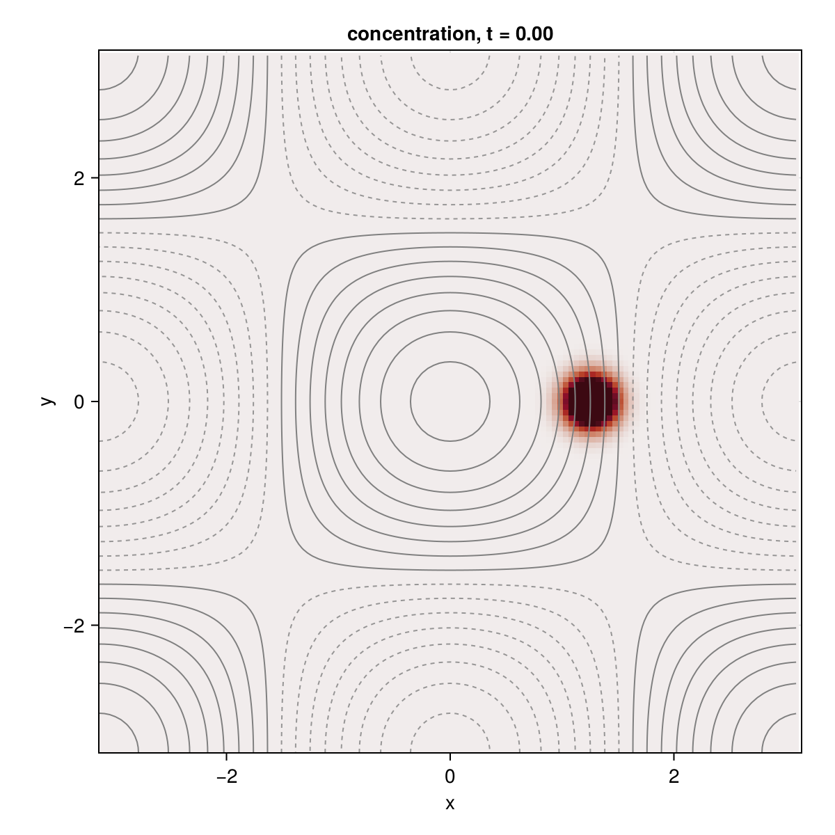

Now we time-step Problem and update the c_anim and title observables as we go to create an animation.

startwalltime = time()

frames = 0:round(Int, nsteps/nsubs)
record(fig, "cellularflow_advection-diffusion.mp4", frames, framerate = 12) do j
   if j % (200 / nsubs) == 0
      log = @sprintf("step: %04d, t: %d, walltime: %.2f min",
                     clock.step, clock.t, (time()-startwalltime)/60)

      println(log)
    end

  c_anim[] = vars.c
  title[] = @sprintf("concentration, t = %.2f", clock.t)

  stepforward!(prob, nsubs)
  TracerAdvectionDiffusion.updatevars!(prob)
end

"cellularflow_advection-diffusion.mp4"

This page was generated using Literate.jl.